Solution Exercise 1

Data Simulation with Monte Carlo Methods

Marko Bachl

University of Hohenheim

Group exercise 1

Exercise 1a. Proving the CLT for a Poisson distribution

• Adapt the code from the examples to check whether the CLT also holds for a Poisson distribution.

  • Random numbers are sampled with rpois(n, lambda), where n is the sample size and lambda is the mean (and also the variance) of the distribution.

  • The population standard deviation is \(\sqrt{\lambda}\).

Solution 1a: Proving the CLT for a Poisson distribution

# Population distribution: Poisson
set.seed(825) # make results reproducible 
lambda = 5
n = 100
mu = lambda
sigma = sqrt(lambda)
ggplot() + 
  stat_function(fun = dpois,
                n = 16,
                xlim = c(0,15),
                args = list(lambda = lambda),
                geom = "bar") + 
  geom_vline(xintercept = mu) + labs(x = NULL)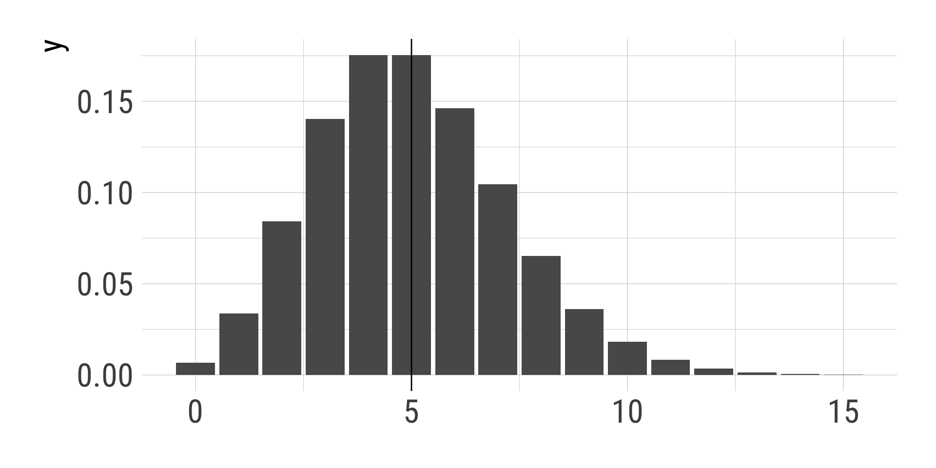

Solution 1a: Proving the CLT for a Poisson distribution

# new function
sim_CLT_pois = function(n, lambda) {
  sims = rpois(n = n, lambda = lambda)
  mean(sims)
}
i = 10000
many_means = map_dbl(1:i, .f = ~ sim_CLT_pois(n = n, lambda = lambda))

Solution 1a: Proving the CLT for a Poisson distribution

mu; mean(many_means)

[1] 5

[1] 4.997543

sigma / sqrt(n); sd(many_means)

[1] 0.2236068

[1] 0.2214916

Solution 1a: Proving the CLT for a Poisson distribution

Show the code

d_many_means = tibble(sim = 1:i, mu_hat = many_means)
d_many_means %>% 
  ggplot(aes(mu_hat)) + geom_histogram() + 
  geom_vline(xintercept = c(mu - sigma / sqrt(n), mu, mu + sigma / sqrt(n))) +
  geom_vline(xintercept = c(mean(many_means)-sd(many_means),
                            mean(many_means),
                            mean(many_means)+sd(many_means)), 
             color = "red", linetype = 2)
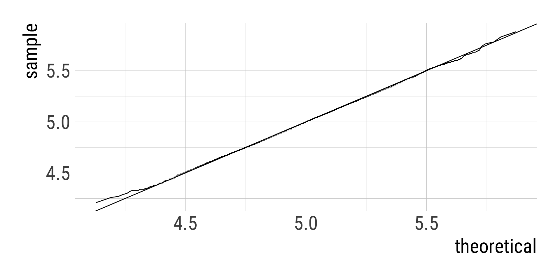
d_many_means %>% 
  ggplot(aes(sample = many_means)) +
  geom_qq(distribution = qnorm, 
          dparams = c(mean = mu, sd = sigma / sqrt(n)), 
          geom = "line") + 
  geom_abline(slope = 1)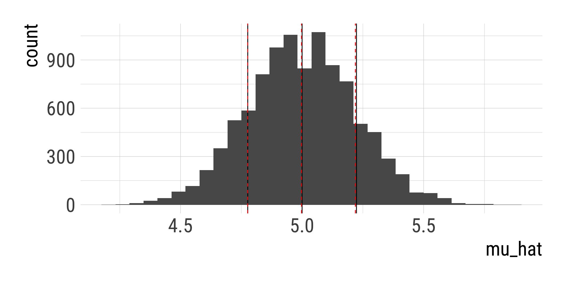

Histogram of sample means

Q-Q-Plot

Exercise 1b. Proving the CLT for any other suitable distribution

• Select another suitable distribution from ?Distributions

  • Read the documentation to understand which arguments must be provided.

  • Find the definition of the population distribution’s standard deviation to calculate the analytical standard deviation of the sampling distribution.

  • Adapt the simulation and analysis code accordingly.

One possible solution for 1b. Proving the CLT for a Student T distribution

set.seed(951) # make results reproducible 
df = 5 # degrees of freedom
n = 100
mu = 0 # Central T
sigma = sqrt(df/(df - 2)) # Standard deviation of a T distribution
ggplot() + 
  stat_function(fun = dt,
                args = list(df = df),
                xlim = c(-3,3)) + 
  geom_vline(xintercept = mu) + labs(x = NULL)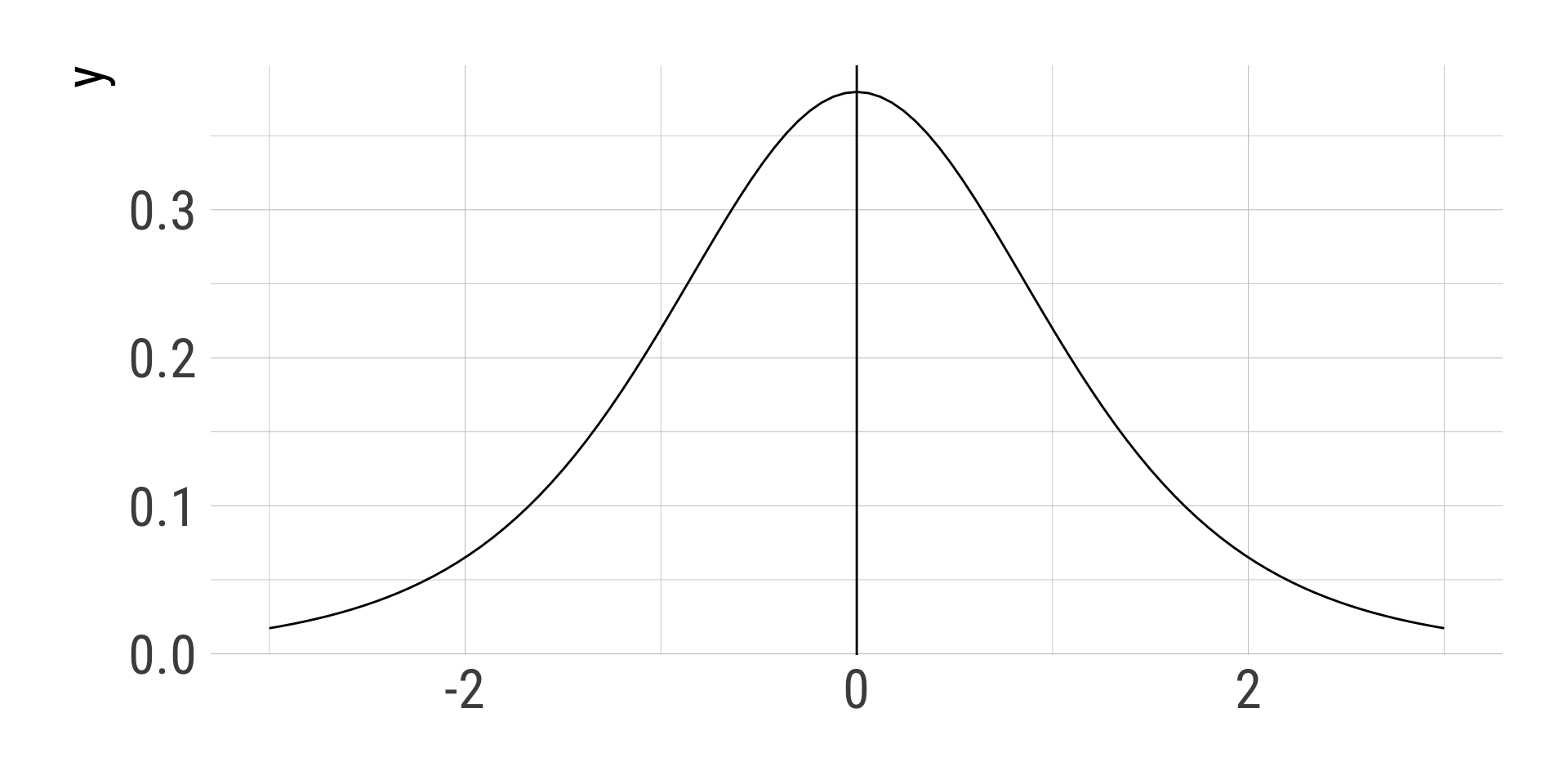

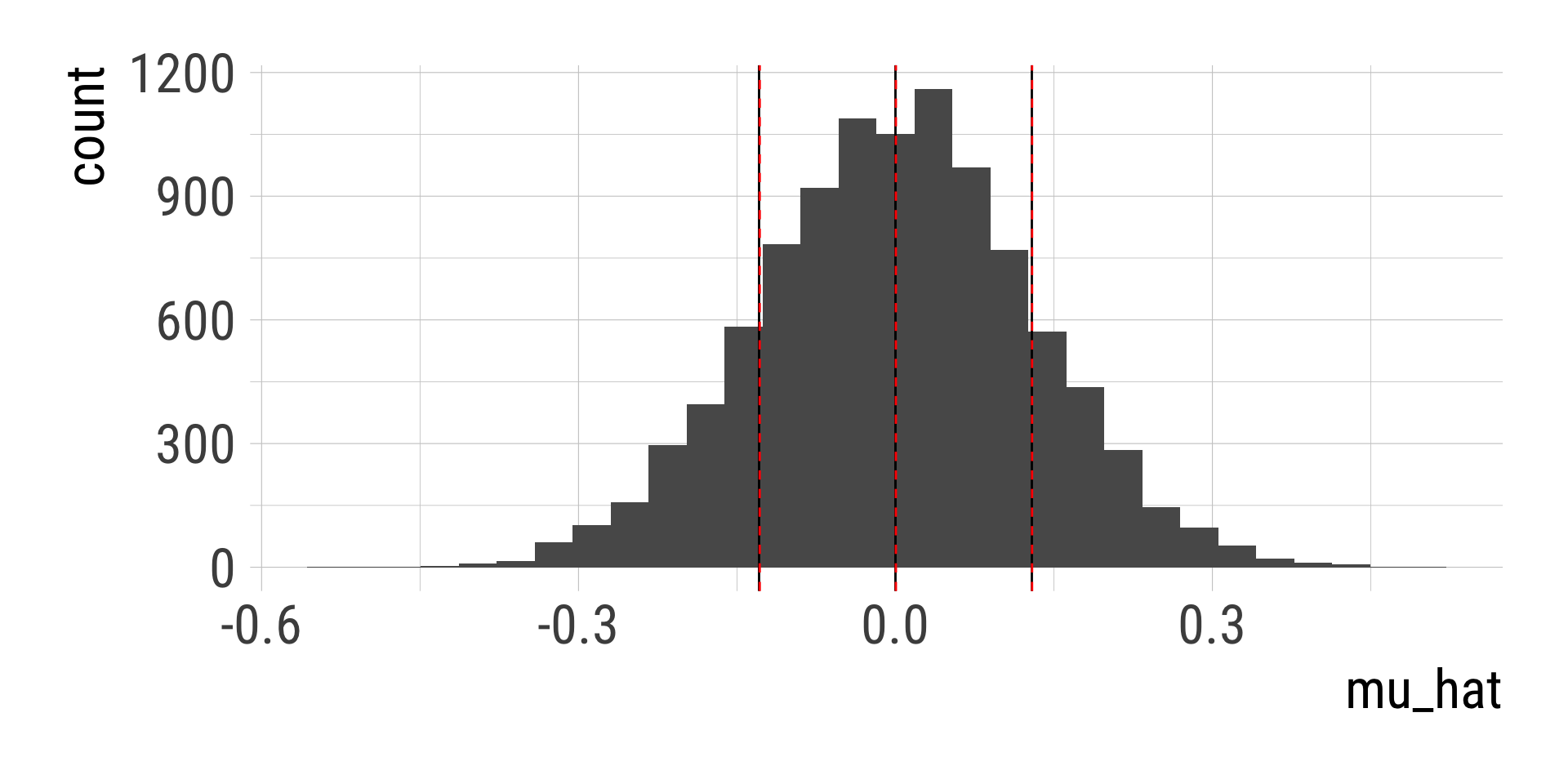
Solution 1b. Proving the CLT for a Student T distribution

# new function
sim_CLT_t = function(n, df) {
  sims = rt(n = n, df = df)
  mean(sims)
}
i = 10000
many_means = map_dbl(1:i, .f = ~ sim_CLT_t(n = n, df = df))

Solution 1b. Proving the CLT for a Student T distribution

mu; mean(many_means)

[1] 0

[1] 0.0004013506

sigma / sqrt(n); sd(many_means)

[1] 0.1290994

[1] 0.1288953

Solution 1b. Proving the CLT for a Student T distribution

Show the code

d_many_means = tibble(sim = 1:i, mu_hat = many_means)
d_many_means %>% 
  ggplot(aes(mu_hat)) + geom_histogram() + 
  geom_vline(xintercept = c(mu - sigma / sqrt(n), mu, mu + sigma / sqrt(n))) +
  geom_vline(xintercept = c(mean(many_means)-sd(many_means),
                            mean(many_means),
                            mean(many_means)+sd(many_means)), 
             color = "red", linetype = 2)
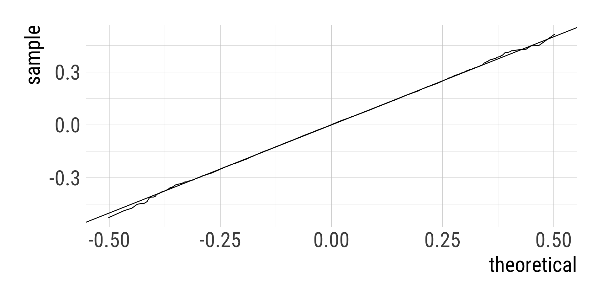
d_many_means %>% 
  ggplot(aes(sample = many_means)) +
  geom_qq(distribution = qnorm, 
          dparams = c(mean = mu, sd = sigma / sqrt(n)), 
          geom = "line") + 
  geom_abline(slope = 1)

Histogram of sample means

Q-Q-Plot