set.seed(28)
n = 150 # fixed total sample size
GR = 2 # n2/n1
n1 = round(n / (GR + 1))
n2 = round(n1 * GR)
sd1 = 1
SDR = 2  # sd2/sd1
sd2 = sd1 * SDR4a) Errors and power — Torturing the t-test
Data Simulation with Monte Carlo Methods
University of Hohenheim
Errors and power — Torturing the t-test
Traktandenliste
Introduction & overview
Monte Carlo Simulation?
Proof by simulation — The Central Limit Theorem (CLT)
Errors and power — Torturing the t-test
Misclassification and bias — Messages mismeasured
Outlook: What’s next?
4. Errors and power — Torturing the t-test
Comparison of Student’s and Welch’s t-tests
A priori power calculation for Welch’s t-test
Student’s t-test & Welch’s t-test
Student’s t-test for two independent means
\(t = \frac{\bar{X}_1 - \bar{X}_2}{s_p \sqrt\frac{2}{n}}\), where \(s_p = \sqrt{\frac{s_{X_1}^2+s_{X_2}^2}{2}}\) and \(df = n_1 + n_2 − 2\)
Welch’s t-test for two independent means
\(t = \frac{\bar{X}_1 - \bar{X}_2}{s_{\bar\Delta}}\), where \({\bar\Delta} = \sqrt{\frac{s_1^2}{n_1} + \frac{s_2^2}{n_2}}\) and \(df = \frac{\left(\frac{s_1^2}{n_1} + \frac{s_2^2}{n_2}\right)^2}{\frac{\left(s_1^2/n_1\right)^2}{n_1-1} + \frac{\left(s_2^2/n_2\right)^2}{n_2-1}}\)
Student’s t-test & Welch’s t-test

Student’s t-test & Welch’s t-test
Old school (AI) advice: Student’s t-test for equal variances, Welch’s t-test for unequal variances.
- Higher power of Student’s t-test if assumptions hold.
Modern advice: Always use Welch’s t-test.
Better if assumptions are violated; not worse if assumptions hold.
e.g., Delacre, M., Lakens, D., & Leys, C. (2017). Why Psychologists Should by Default Use Welch’s t-test Instead of Student’s t-test. International Review of Social Psychology, 30(1). https://doi.org/10.5334/irsp.82
For those who don’t care about t-tests: Idea also applies to heteroskedasticity-consistent standard errors.
First Simulation study: False discoveries
Question: What is the goal of the simulation?
- Comparison of Student’s and Welch’s t-tests
Quantities of interest: What is measured in the simulation?
- \(\alpha\) error rate of the tests
Evaluation strategy: How are the quantities assessed?
- Comparison of empirical distribution of p-values with theoretical distribution under the Null hypothesis
Conditions: Which characteristics of the data generating model will be varied?
- Group size ratio; Standard deviation ratio
Data generating model: How are the data simulated?
- Random draws from normal distributions with equal means, but different group sizes and standard deviations
Practical considerations
How does the
t.test()work in R?Which parameters and functions do we need for generating the data?
How do we implement the experimental design for the simulation study?
How do we run the simulation?
How do we assess and visualize the results?
One simulation: Parameters
Two factors:
Group sizes: Equal or unequal?
Group standard deviations: Equal or unequal?
Implementation with ratios and fixed total sample size.
One simulation: t-tests
g1 = rnorm(n = n1, mean = 0, sd = sd1)
g2 = rnorm(n = n2, mean = 0, sd = sd2)
t.test(g1, g2) # Welch (default)
t.test(g1, g2, var.equal = TRUE) # Student
    Welch Two Sample t-test

data:  g1 and g2
t = 0.74022, df = 147.94, p-value = 0.4603
alternative hypothesis: true difference in means is not equal to 0
95 percent confidence interval:
 -0.3198803  0.7030466
sample estimates:
  mean of x   mean of y
-0.09838857 -0.28997168
    Two Sample t-test

data:  g1 and g2
t = 0.60009, df = 148, p-value = 0.5494
alternative hypothesis: true difference in means is not equal to 0
95 percent confidence interval:
 -0.4393035  0.8224698
sample estimates:
  mean of x   mean of y
-0.09838857 -0.28997168
Inspect the output of t.test()
List of 10
 $ statistic  : Named num 0.74
  ..- attr(*, "names")= chr "t"
 $ parameter  : Named num 148
  ..- attr(*, "names")= chr "df"
 $ p.value    : num 0.46
 $ conf.int   : num [1:2] -0.32 0.703
  ..- attr(*, "conf.level")= num 0.95
 $ estimate   : Named num [1:2] -0.0984 -0.29
  ..- attr(*, "names")= chr [1:2] "mean of x" "mean of y"
 $ null.value : Named num 0
  ..- attr(*, "names")= chr "difference in means"
 $ stderr     : num 0.259
 $ alternative: chr "two.sided"
 $ method     : chr "Welch Two Sample t-test"
 $ data.name  : chr "g1 and g2"
- attr(*, "class")= chr "htest"Wrap it into a function
sim_ttest = function(GR = 1, SDR = 1, n = 150) {
  n1 = round(n / (GR + 1))
  n2 = round(n1 * GR)
  sd1 = 1
  sd2 = sd1 * SDR
  g1 = rnorm(n = n1, mean = 0, sd = sd1)
  g2 = rnorm(n = n2, mean = 0, sd = sd2)
  Welch = t.test(g1, g2)$p.value
  Student = t.test(g1, g2, var.equal = TRUE)$p.value
  res = lst(Welch, Student)
  return(res)
}
Call the function once
Setup of experimental conditions
expand_grid()is the tidy implementation ofbase::expand.grid().- Creates a data frame from all combinations of the supplied vectors.
Setup of experimental conditions
- Two between-simulation factors:
GRandSDR
Setup of experimental conditions
| condition | GR | SDR | implies |
|---|---|---|---|
| 1 | 1 | 0.5 | n1 = 75, n2 = 75, sd1 = 1, sd2 = 0.5 |
| 2 | 1 | 1.0 | n1 = 75, n2 = 75, sd1 = 1, sd2 = 1 |
| 3 | 1 | 2.0 | n1 = 75, n2 = 75, sd1 = 1, sd2 = 2 |
| 4 | 2 | 0.5 | n1 = 50, n2 = 100, sd1 = 1, sd2 = 0.5 |
| 5 | 2 | 1.0 | n1 = 50, n2 = 100, sd1 = 1, sd2 = 1 |
| 6 | 2 | 2.0 | n1 = 50, n2 = 100, sd1 = 1, sd2 = 2 |
Run simulation experiment
set.seed(689)
i = 10000 # number of sim runs per condition
tic() # simple way to measure wall time
sims = map_dfr(1:i, ~ conditions) %>% # each condition i times
  rowid_to_column(var = "sim") %>% # within simulation comparison
  rowwise() %>%
  mutate(p.value = list(sim_ttest(GR = GR, SDR = SDR))) %>%
  unnest_longer(p.value, indices_to = "method")
toc() # simple way to measure wall time
14.949 sec elapsedInspect simulated data
# A tibble: 120,000 × 6
     sim condition    GR   SDR p.value method
   <int>     <int> <dbl> <dbl>   <dbl> <chr>
 1     1         1     1   0.5 0.345   Welch
 2     1         1     1   0.5 0.344   Student
 3     2         2     1   1   0.534   Welch
 4     2         2     1   1   0.534   Student
 5     3         3     1   2   0.647   Welch
 6     3         3     1   2   0.647   Student
 7     4         4     2   0.5 0.00985 Welch
 8     4         4     2   0.5 0.00224 Student
 9     5         5     2   1   0.602   Welch
10     5         5     2   1   0.614   Student
# … with 119,990 more rows
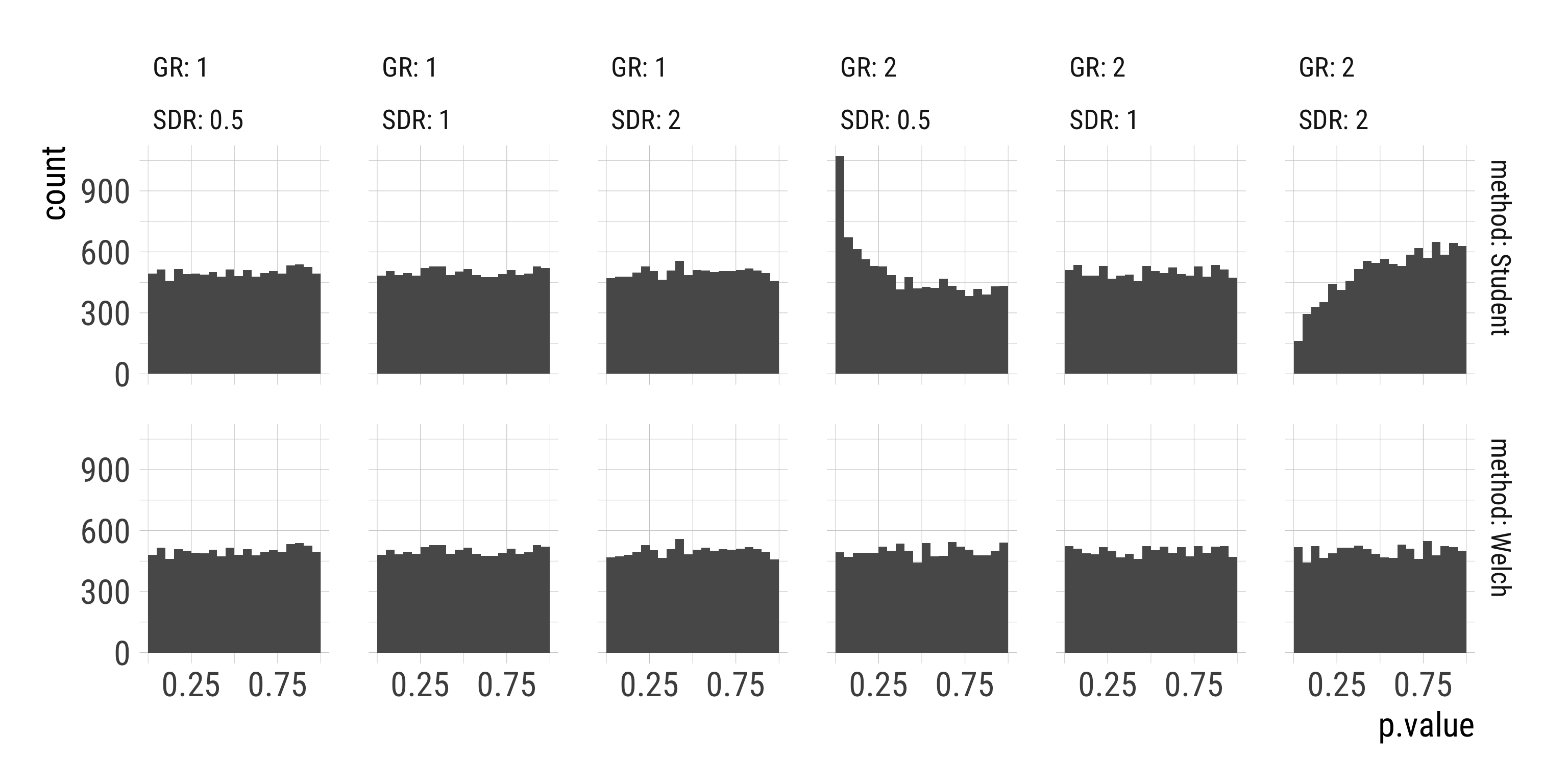
Results: Histogram of p-values
- Distribution of p-values under the Null hypothesis should be \(\sf{Uniform}(0, 1)\).
Results: Histogram of p-values

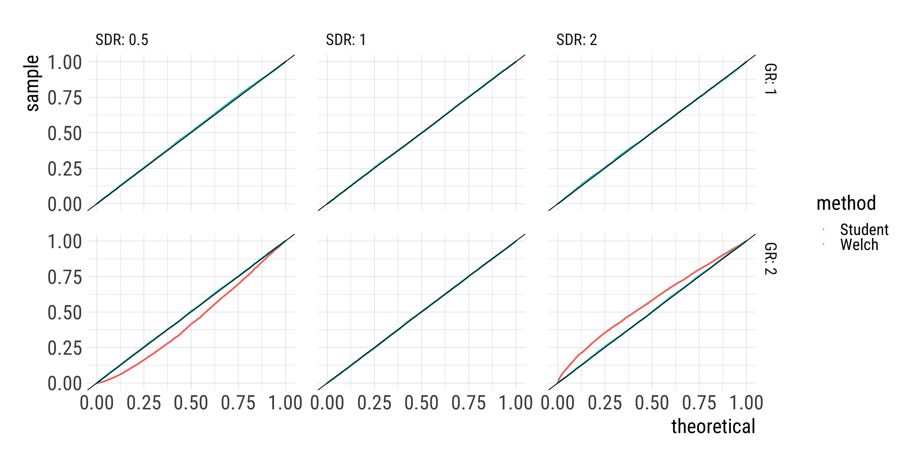
Results: Q-Q-plot of p-values
- Distribution of p-values under the Null hypothesis should be \(\sf{Uniform}(0, 1)\).
Results: Q-Q-plot of p-values

Results: Looking at the relevant tail
| GR | SDR | method | P_p001 | P_p01 | P_p05 |
|---|---|---|---|---|---|
| 1 | 0.5 | Student | 0.001 | 0.010 | 0.049 |
| 1 | 0.5 | Welch | 0.001 | 0.010 | 0.048 |
| 1 | 1.0 | Student | 0.000 | 0.010 | 0.048 |
| 1 | 1.0 | Welch | 0.000 | 0.010 | 0.048 |
| 1 | 2.0 | Student | 0.001 | 0.011 | 0.047 |
| 1 | 2.0 | Welch | 0.001 | 0.010 | 0.047 |
| 2 | 0.5 | Student | 0.008 | 0.034 | 0.107 |
| 2 | 0.5 | Welch | 0.002 | 0.010 | 0.049 |
| 2 | 1.0 | Student | 0.001 | 0.010 | 0.051 |
| 2 | 1.0 | Welch | 0.000 | 0.010 | 0.052 |
| 2 | 2.0 | Student | 0.000 | 0.002 | 0.016 |
| 2 | 2.0 | Welch | 0.001 | 0.009 | 0.052 |
Questions?
Group exercise 2
Exercise 2: Welch’s t-test for count data
Part 1: False discovery rates
It is generally recommended to model count outcomes (e.g., number of likes of social media posts) with Poisson models (or negative binomial models, but that’s for another simulation).
However, if we only want to compare two groups on a count outcome, Welch’s t-test might be an easier option and should also do well:
- The mean is a consistent estimator of the rate parameter (CLT; see exercise 1a).
- Welch’s t-test is robust if the group standard deviations are unequal, which, by definition, would be the case if the counted event occurred at different rates in the two groups.
Exercise 2a: False discovery rates
We can test this assumption by simulation, similar to the comparison of Student’s and Welch’s t-test. More specifically, we first want to compare the false discovery rates of
- Student’s t-test,
- Welch’s t-test, and
- Poisson regression with a dummy predictor
if the true data generating process is drawing from a Poisson distribution.
Extend and adapt the previous simulation.
Exercise 2a: Help
Expand if you need help.
Don’t expand if you want to figure it out by yourself.
Scroll down if you need more help on later steps.
Sample from a Poisson distribution
Poisson regression
Data format for Poisson regression
Extract p-value from fitted Poisson regression object
Complete simulation function
Code
# No standard deviation ratio any more because SD fixed at sqrt(lambda)
# M_diff not necessary at this stage, but useful later
sim_ttest_glm = function(n = 200, GR = 1, lambda1 = 1, M_diff = 0) {
  n1 = round(n / (GR + 1))
  n2 = round(n1 * GR)
  lambda2 = lambda1 + M_diff
  g1 = rpois(n = n1, lambda = lambda1)
  g2 = rpois(n = n2, lambda = lambda2)
  Welch = t.test(g1, g2)$p.value
  Student = t.test(g1, g2, var.equal = TRUE)$p.value
  GLM = glm(outcome ~ group,
            data = data.frame(outcome = c(g1, g2),
                              group = c(rep("g1", n1), rep("g2", n2))),
            family = poisson)
  res = lst(Welch, Student, GLM = coef(summary(GLM))[2, 4])
  return(res)
}
Conditions
Run simulation
Code
# use smaller i for now because additional glm() needs time
set.seed(35)
i = 1000
tic()
sims = map_dfr(1:i, ~ conditions) %>%
  rowid_to_column(var = "sim") %>%
  rowwise() %>%
  mutate(p.value = list(sim_ttest_glm(n = n, M_diff = M_diff,
                                 GR = GR, lambda1 = lambda1))) %>%
  unnest_longer(p.value, indices_to = "method")
toc()
Plots
Code
# Histogram of p-values
sims %>%
  ggplot(aes(p.value)) +
  geom_histogram(binwidth = 0.1, boundary = 0) +
  facet_grid(method ~ lambda1 + GR, labeller = label_both) +
  scale_x_continuous(breaks = c(1, 3)/4)
# QQ-Plot of p-values
sims %>%
  ggplot(aes(sample = p.value, color = method)) +
  geom_qq(distribution = stats::qunif, geom = "line") +
  geom_abline(slope = 1) +
  facet_grid(GR ~ lambda1, labeller = label_both)
# Rates of p < .05
sims %>%
  group_by(GR, lambda1, method) %>%
  summarise(P_p05 = mean(p.value < 0.05)) %>%
  ggplot(aes(factor(GR), P_p05, color = method, group = method)) +
  geom_point() + geom_line() +
  geom_hline(yintercept = 0.05, linetype = 2) +
  facet_wrap(vars(lambda1), labeller = label_both) +
  labs(x = "Group size ratio", y = "Proportion p < 0.05")