Solution Exercise 3

Data Simulation with Monte Carlo Methods

Marko Bachl

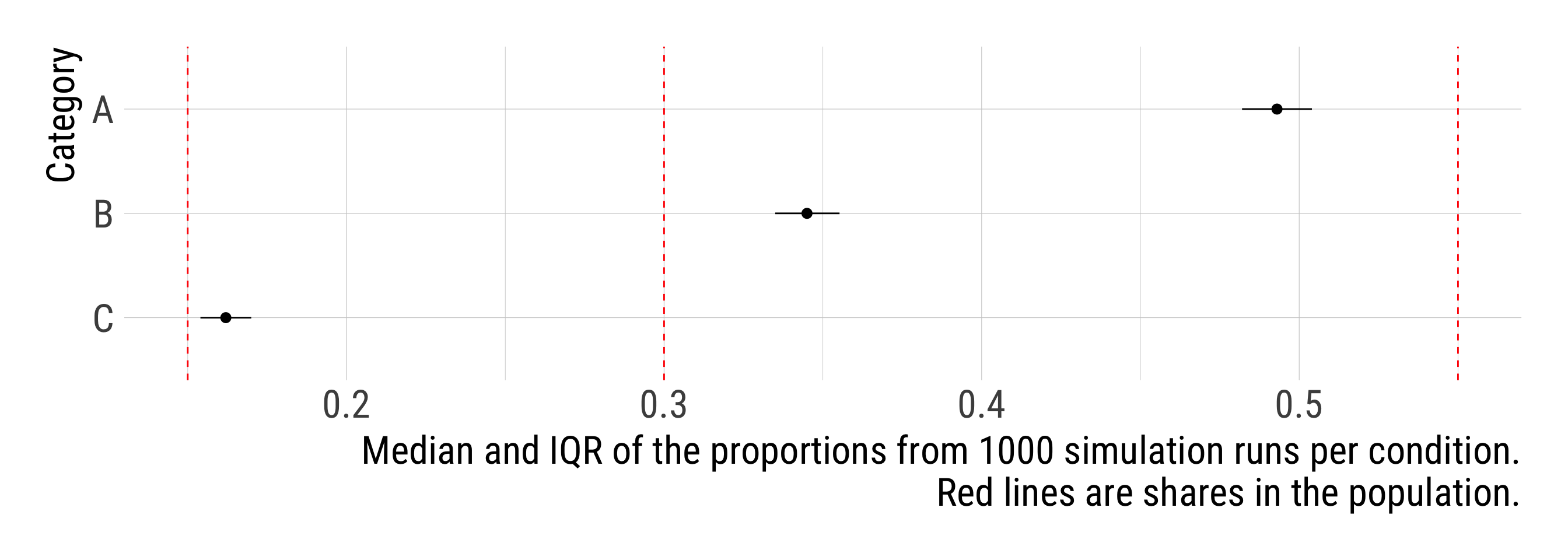
University of Hohenheim

Group exercise 3

Group exercise 3

Try one (or more) of the following adaptions of the Monte Carlo studies on misclassification:

1. Change the first simulation so that the misclassification probabilities to allow for different patterns accuracies and errors: varying difficulties of the categories, systematic confusion of some categories.

2. Investigate the consequences of misclassification error for an analysis of two binary variables which were both measured with misclassification error.

A) Different misclassification probabilities

A simple example with systematic confusion for illustrative purposes

• Only one fixed confusion matrix
  • True A more likely to be confused with B
  • C less accurate

misclass_prob = matrix(c(
  .80, .10, .15,
  .15, .80, .15,
  .05, .10, .70
), nrow = 3, byrow = TRUE,
dimnames = list(LETTERS[1:3], LETTERS[1:3]))
misclass_prob

     A   B    C
A 0.80 0.1 0.15
B 0.15 0.8 0.15
C 0.05 0.1 0.70

Adapted simulation function

Misclassification matrix as argument

sim_misclass = function(pop_dist = c(0.55, 0.3, 0.1, 0.05),
                        n = 1000,
                        misclass_prob = misclass_prob) {
  # Population
  k = length(pop_dist)
  categories = LETTERS[1:k]
  
  # Sample
  sample_true = sample(x = categories, 
                       size = n, 
                       replace = TRUE, 
                       prob = pop_dist) %>% 
    factor(levels = categories) %>% 
    sort()
  freq_true = sample_true %>% 
    table() %>% 
    prop.table()
  
  # Misclassification
  sample_obs = table(sample_true) %>%  
    imap(~ sample(categories,
                  size = .x, replace = TRUE, 
                  prob = misclass_prob[, .y])) %>%
    unlist(use.names = FALSE) %>% 
    factor(levels = categories)
  freq_obs = sample_obs %>% 
    table() %>% 
    prop.table()
  
  # Error summary
  rmse = sqrt(mean((pop_dist - freq_obs)^2))
  
  # Output
  out = lst(freq_true, freq_obs, rmse)
  out
}

Condition

• No experiment, just one condition for illustration

conditions = expand_grid(
  pop_dist = list(c(0.55, 0.3, 0.15)),
  n = 1000,
  misclass_prob = list(misclass_prob)
) %>% 
  rowid_to_column(var = "condition")
conditions

# A tibble: 1 × 4
  condition pop_dist      n misclass_prob
      <int> <list>    <dbl> <list>       
1         1 <dbl [3]>  1000 <dbl [3 × 3]>

Run simulation

i = 1000 # less simulations to save some workshop time 
set.seed(40)
tic()
sims = map_dfr(1:i, ~ conditions) %>%
  rowid_to_column(var = "sim") %>%
  rowwise() %>%
  mutate(res = list(sim_misclass(pop_dist = pop_dist, 
                                 n = n, misclass_prob = misclass_prob)))
toc()

0.711 sec elapsed

Results

Show the code

sims %>% 
  ungroup() %>% 
  unnest_wider(res) %>% 
  unnest_longer(freq_obs, indices_to = "category") %>% 
  group_by(category) %>%
  summarise(Q = list(quantile(freq_obs, probs = c(0.25, 0.5, 0.75)))) %>%
  unnest_wider(Q) %>%
  ggplot(aes(`50%`, fct_rev(category),
             xmin = `25%`, xmax = `75%`)) +
  geom_pointrange() +
  geom_vline(xintercept = unlist(conditions$pop_dist), color = "red", linetype = 2) + 
  labs(x = str_glue("Median and IQR of the proportions from {i} simulation runs per condition.\nRed lines are shares in the population."),
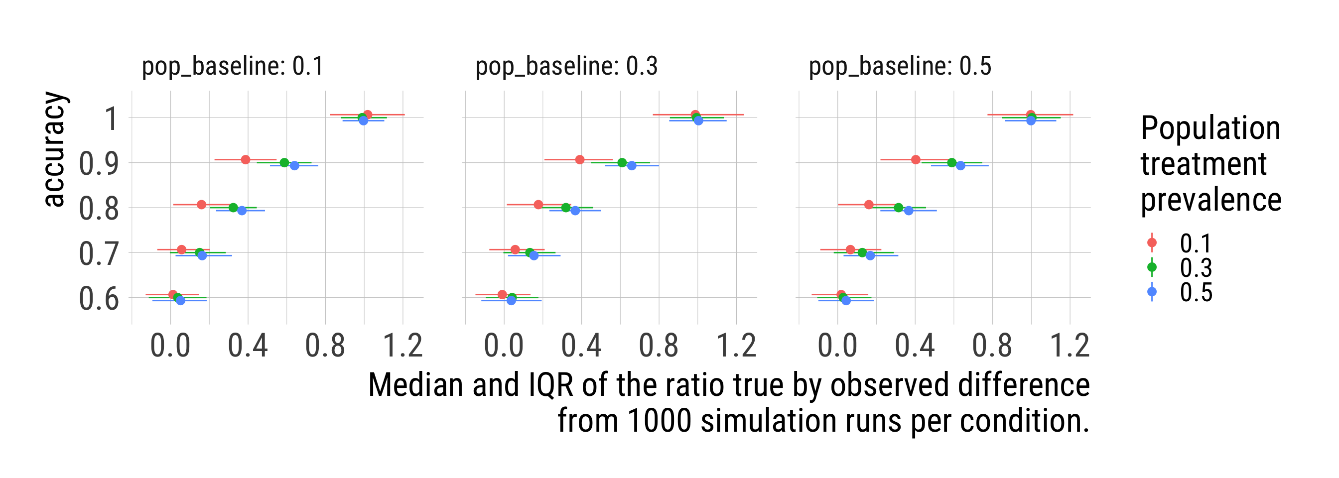
       y = "Category")

b) Two misclassified binary variables

• This could be done with a close adaption of the second simulation, i.e., using the sample() function for data generation and misclassification.

• However, simulation with binary variables is much simpler and more efficient with rbinom().

• The following solution shows the latter option.

One simulation: Misclassification-free sample of the independent variable

• Draw a sample of size n of the independent variable with population prevalence pop_dist_x.

set.seed(91)
n = 1000
pop_dist_x = 0.5
sample_x_true = rbinom(n = n, 
                         size = 1, 
                         prob = pop_dist_x)
prop.table(table(sample_x_true))

sample_x_true
    0     1 
0.507 0.493 

One simulation: Misclassification-free sample of the outcome

• pop_baseline: Probability of the outcome in the baseline group, i.e., sample_x_true == 0

• pop_difference: Difference between probabilities of the outcome in the baseline and treatment groups

• logit_pop_baseline: logit (i.e., \(log(x / (1 - x)\)) of the baseline probability

• pop_oddsratio: Odds ratio of the outcome in the baseline and treatment groups

• pop_logodds: log(odds)

• outcomes_true: Draw outcome n times from a binomial distribution, where the success probability is a function of the baseline probability and the log odds of the probabilities in the baseline and treatment groups

pop_baseline = 0.5
pop_difference = 0.1
logit_pop_baseline = log(pop_baseline / (1 - pop_baseline))
pop_oddsratio = ((pop_baseline + pop_difference) / (1 - (pop_baseline + pop_difference))) /
  (pop_baseline / (1 - pop_baseline))
pop_logodds = log(pop_oddsratio)
outcomes_true = rbinom(n = n, size = 1,
                         prob = 1 / (1 + exp(- (logit_pop_baseline + pop_logodds * sample_x_true))))
prop.table(table(outcomes_true, sample_x_true), margin = 2) %>% round(2)

             sample_x_true
outcomes_true    0    1
            0 0.53 0.40
            1 0.47 0.60

One simulation: Misclassification of the variables

• Each observation is classified correctly with probability of accuracy, regardless of its true value.

• correct_ are vectors of length n which record whether an observation was misclassified (1) or not (0).

• abs(_true - correct_) switches the values for all observations which are noted as misclassified, correct_ == 1.

# Misclassification probabilities
accuracy = 0.8
correct_x = rbinom(n = n, size = 1, 
                   prob = (1 - accuracy))
correct_outcome = rbinom(n = n, size = 1, 
                         prob = (1 - accuracy))

# Misclassification
sample_x_obs = abs(sample_x_true - correct_x)
outcomes_obs = abs(outcomes_true - correct_outcome)
mean(sample_x_obs == sample_x_true); mean(outcomes_obs == outcomes_true)

[1] 0.797

[1] 0.801

One simulation: Quantities for evaluation

• We use Welch’s t-test to estimate the differences in the observed outcome between the observed groups.

• We extract the p-value, p_obs, for computing statistical power.

• We extract the estimated absolute difference, diff_obs, and its ratio to the true population difference, diff_obs_rel.

  t_res = t.test(outcomes_obs ~ sample_x_obs)
  (p_obs = t_res$p.value)

[1] 0.06787792

  (diff_obs = unname(diff(t_res$estimate)))

[1] 0.05773169

  (diff_obs_rel = diff_obs / pop_difference)

[1] 0.5773169

Wrap it into a function

sim_misclass_binary = function(pop_dist_x = 0.5,
                               pop_baseline = 0.5,
                               pop_difference = 0.1,
                               n = 1000,
                               accuracy = 0.8) {
  # Population
  logit_pop_baseline = log(pop_baseline / (1 - pop_baseline))
  pop_oddsratio = ((pop_baseline + pop_difference) / (1 - (pop_baseline + pop_difference))) /
    (pop_baseline / (1 - pop_baseline))
  pop_logodds = log(pop_oddsratio)
  
  # True sample
  sample_x_true = rbinom(n = n, 
                         size = 1, 
                         prob = pop_dist_x)
  outcomes_true = rbinom(n = n, size = 1,
                         prob = 1 / (1 + exp(- (logit_pop_baseline + pop_logodds * sample_x_true))))
  
  # Misclassification probabilities
  correct_x = rbinom(n = n, size = 1, prob = (1 - accuracy))
  correct_outcome = rbinom(n = n, size = 1, prob = (1 - accuracy))
  
  # Misclassification
  sample_x_obs = abs(sample_x_true - correct_x)
  outcomes_obs = abs(outcomes_true - correct_outcome)

  # Model
  t_res = t.test(outcomes_obs ~ sample_x_obs)
  p_obs = t_res$p.value
  diff_obs = unname(diff(t_res$estimate))
  diff_obs_rel = diff_obs / pop_difference
  
  
  # Output
  out = lst(p_obs, diff_obs, diff_obs_rel)
  return(out)
}

Conditions

• We vary the prevalence of the treatment in the population, pop_dist_x, the prevalence of the outcome in the baseline group, pop_baseline, and, most importantly, the accuracy of the measurements.

conditions = expand_grid(
  pop_dist_x = c(.1, .3, .5),
  pop_baseline = c(.1, .3, .5),
  pop_difference = 0.15,
  n = 1000,
  accuracy = seq(from = 0.6, to = 1, by = 0.1)
) %>% 
  rowid_to_column(var = "condition")
conditions

# A tibble: 45 × 6
   condition pop_dist_x pop_baseline pop_difference     n accuracy
       <int>      <dbl>        <dbl>          <dbl> <dbl>    <dbl>
 1         1        0.1          0.1           0.15  1000      0.6
 2         2        0.1          0.1           0.15  1000      0.7
 3         3        0.1          0.1           0.15  1000      0.8
 4         4        0.1          0.1           0.15  1000      0.9
 5         5        0.1          0.1           0.15  1000      1  
 6         6        0.1          0.3           0.15  1000      0.6
 7         7        0.1          0.3           0.15  1000      0.7
 8         8        0.1          0.3           0.15  1000      0.8
 9         9        0.1          0.3           0.15  1000      0.9
10        10        0.1          0.3           0.15  1000      1  
# … with 35 more rows

Run simulation

i = 1000 # less simulations to save some workshop time 
set.seed(40)
tic()
sims = map_dfr(1:i, ~ conditions) %>%
  rowid_to_column(var = "sim") %>%
  rowwise() %>%
  mutate(res = list(sim_misclass_binary(pop_dist_x = pop_dist_x, 
                                        pop_baseline = pop_baseline,
                                        pop_difference = pop_difference,
                                        n = n, accuracy = accuracy)))
toc()

43.462 sec elapsed

Results: Recovered difference

Show the code

sims %>% 
  ungroup() %>% 
  unnest_wider(res) %>% 
  group_by(accuracy, pop_baseline, pop_dist_x) %>% 
  summarise(Q = list(quantile(diff_obs_rel, probs = c(0.25, 0.5, 0.75)))) %>% 
  unnest_wider(Q) %>% 
  ggplot(aes(`50%`, factor(accuracy), color = factor(pop_dist_x),
             xmin = `25%`, xmax = `75%`)) +
  geom_pointrange(position = position_dodge(width = -.2)) +
  facet_wrap(vars(pop_baseline), labeller = "label_both") + 
  labs(y = "accuracy",
       x = str_glue("Median and IQR of the ratio true by observed difference\nfrom {i} simulation runs per condition."),
       color = "Population\ntreatment\nprevalence")

Results: Power

Show the code

sims %>% 
  ungroup() %>% 
  unnest_wider(res) %>% 
  group_by(accuracy, pop_baseline, pop_dist_x) %>% 
  summarise(P_p05 = mean(p_obs < 0.05)) %>% 
  ggplot(aes(accuracy, P_p05, color = factor(pop_dist_x))) + 
  geom_point() + geom_line() +
  facet_wrap(vars(pop_baseline), labeller = "label_both") + 
  labs(y = "Power at p < .05", color = "Population\ntreatment\nprevalence")